Quick start examples

We will now show how can we compute a spectrum using pyrh. The user should be familiar with RH code in general. The basic usage is done through *.input files of RH and user should use these as he would use them when calling RH from a shell.

Open now the examples/synth.py script in your favourite editor.

We will first load in the atmospheric model. Here we will use FAL C atmosheric model:

import numpy as np
import matplotlib.pyplot as plt
import pyrh

def spinor2multi(atm):
        """
        Casting from SPINOR type atmosphere structure to MULTI type structure.
        """
        from scipy.constants import k
        new = np.empty(atm.shape, dtype=np.float64)

        new[0] = atm[0]
        new[1] = atm[2]
        # electron number dnesity
        new[2] = atm[4]/10/k/atm[2] / 1e6 # [1/cm3]
        new[3] = atm[9]/1e5
        new[4] = atm[8]/1e5
        # magnetic field vector: strength, inclination and azimuth
        new[5] = atm[7]
        new[6] = atm[-2]
        new[7] = atm[-1]
        # total hydrogen number density
        new[8] = (atm[3] - atm[4])/10/k/atm[2] / 1e6 / 1.26 # [1/cm3]

        return new

atmos = np.loadtxt("falc.dat", skiprows=1)
atmos = np.array(atmos.T, dtype=np.float64)
atmos= spinor2multi(atmos)

Since the atmospheric model is given in SPINOR like format, first we had to convert it into MULTI type format (more about atmospheric model structure in …).

Now, we define couple of variables to configure RH setup:

# path to the *.input files
cwd = "."

# mu angle for which to compute the spectrum
mu = 1.0

# type of atmosphere stratification:
# 0 -- optical depth @ 500nm
# 1 -- mass density [cm2/g]
# 2 -- height [km]
atm_scale = 0

Parameter cwd describes the relative path to a location where .*input files are stored. These are going to be read by RH.

Further, we set up the wavelength grid for which we are synthesizing the spectrum. We will synthesize Fe I 6301 and 6302 line pair, therefore:

# wavelength samples for which to compute the spectrum (in nm) in vacuum
wave = np.linspace(630.0, 630.35, num=251) + 0.2

To compute a spectrum, we will invoke a method pyrh.compute1d() for given set of input parameters as:

spec = pyrh.compute1d(cwd, mu, atm_scale, atmos, wave)
spec = np.array(spec, dtype=np.float64)

And the final product is:

plt.plot(wave, spec[0]*1e8)
plt.xlabel("Wavelength in vacuum [nm]")
plt.ylabel(r"Intensity [10$^{-8}$ W/Hz/srad/m$^2$]")
plt.xlim([wave[0], wave[-1]])
plt.show()

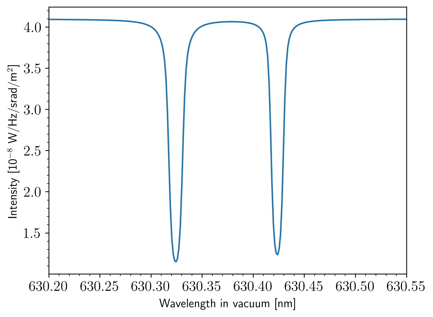
Voila!